Performing Result Set Aggregate Calculations
All of the SELECT statements shown thus far have produced detail rows where each row of the result set corresponds to a single row from the table (a base table or table formed from the set of joined tables in the FROM clause). There are often times when you want to perform a calculation on one or more columns from a related set of rows returning only a summary row that includes the calculation result. The set of rows over which the calculations are performed is called the aggregate. The SELECT statement GROUP BY clause is used to identify the column or columns that define each aggregate—those rows that have identical group by column values. Five built-in aggregate functions are provided in SQL as defined in the table below.
| Function | Description |
|---|---|
| COUNT | Returns the number (distinct) of rows in the aggregate. |
| SUM | Returns the sum of the (distinct) values of expression in the aggregate. |
| AVG | Returns the average of the (distinct) values of expression in the aggregate. |
| MIN | Returns the minimum expression value in the aggregate. |
| MAX | Returns the maximum expression value in the aggregate. |
| EVERY | Returns true if cond_expr is true for every row in the aggregate. |
| ANY/SOME | Returns true if cond_expr is true for at least one row in the aggregate. |
| INVAR | Checks that the value of expressions is invariant (i.e., does not change) within each aggregate. |
| VAR_POP | Computes the population variance over each aggregate. |
| var_samp | Computes the sample variance over each aggregate. |
| stddev_pop | Computes the population standard deviation over each aggregate. |
| stddev_samp | Computes the sample standard deviation over each aggregate. |
The complete syntax for the SELECT statement including GROUP BY is as follows.
select_stmt:
          SELECT [DISTINCT] select_item[, select_item]...
               FROM table_ref [, table_ref]…
               [WHERE conditional_expr]
               [GROUP BY sort_col [, sort_col]… [HAVING conditional_expr] ]
               [ORDER BY sort_col [ASC | DESC] [, sort_col [ASC | DESC]]…]
table_ref:
table_spec | table_joinsort_col:
num | column_vartable_join:
table_ref NATURAL [INNER | {LEFT | RIGHT} [OUTER]] JOIN table_primary
| table_ref [INNER | {LEFT | RIGHT} [OUTER]] JOIN table_primary
[USING ( column_name[, column_name]...) | ON conditional_expr]
select_item:
          named_expr
     |    [table_name.]*
named_expr:
[HIDE] {column_var | value_expr} [[AS] alias_name]arith_expr: /* involving only numeric operands and operations */
operand [{+ | - | * | /} operand]…operand:
constant | column_var | numeric_function | aggregate_fcn
| {+ | -} operand aggregate_fcn:
calc_fcn_name ( [DISTINCT] arith_expr )
| COUNT{* | column_var })
| {EVERY | ANY | SOME} ( conditional_expr )
| {MIN | MAX | INVAR} (value_expr)
| agg_udf_name( [DISTINCT] value_expr)
calc_fcn_name:
          SUM | AVG | VAR_SAMP | VAR_POP | STDDEV_SAMP | STDDEV_POP
To illustrate the basic operation of aggregate calculations, consider the following example which computes the total sales for each bookshop account manager.
select name, count(*), sum(price)
    from (acctmgr join patron using(mgrid)) natural join sale natural join book
    group by 1;

NAME                        COUNT(*)              SUM(PRICE)
Doel, Frank                        5                   31745
Fox, Joe                          19                   95500
Kelly, Kathleen                   14                   67350
Kralik, Alfred                    18                   72685
Noble, Barney                      6                  234700
Novac, Klara                      21                  221650
Zonn, Amy                          9                   15660
The FROM clause needs a little explanation. A natural join between acctmgr and patron cannot be used because besides the mgrid column which is the correct join column both tables have a column called name which is not a legitimate join column as they never contain the same value. So the USING clause is specified to identify the particular common column name on which to form the join.
The count(*) give the number of detail rows (i.e., sold books) in the aggregate for each account manager. The sum(price) gives the total of all of the price values in the aggregate for each account manager.
You can see all of the detail rows that were used in the aggregate calculations by issuing the following query.
select name, price
    from (acctmgr join patron using(mgrid)) natural join sale natural join book
    order by 1;

NAME                            PRICE
Doel, Frank                     25000
Doel, Frank                       750
Doel, Frank                      2500
Doel, Frank                       995
Doel, Frank                      2500
Fox, Joe                         3500
Fox, Joe                        12500
Fox, Joe                          750
Fox, Joe                         1200
	...
Zonn, Amy                        1250
Zonn, Amy                        1200
Zonn, Amy                        4375
Zonn, Amy                         750
Zonn, Amy                         325
Figure 7 illustrates how aggregate calculations are performed on the detail rows that are retrieved.
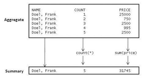
Figure 7. Group By Aggregate Calculations
The WHERE clause is used to restrict the detail rows that form the aggregate to only those rows for which the WHERE conditional expression is true. The HAVING clause is used to restrict result rows that contain the summary aggregate calculations to only those result rows for which the HAVING conditional expression is true.
The following query returns those western state sponsors which have received more than 3/4 billion dollars in funding from the NSF between the years shown.
select
    name,
    invar(state) "state",
    year(min(award_date)) first_year,
    year(max(award_date)) last_year,
    convert(sum(amount), char, 15, "$#,#") funding_total
from sponsor, award where sponsor_nm = name
 	and state in ("AZ","CA","CO","ID","MT","NM","NV","OR","UT","WA","WY")
group by name
having sum(amount) > 750000000.00;

name                       western state first_year last_year   funding_total
California Inst of Tech    CA                  1990      2003    $900,522,261
UCAR                       CO                  1992      2003    $781,735,361
Figure 8 below shows how this query is processed.
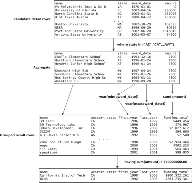
Figure 8. Aggregate Computation with Having Clause
NSF Gender Study Example
The next example is from the NSF awards database. This is a rather involved example that shows how you can use SQL to do analytical studies based on historical data contained in a database. The conclusions that are given are the author's own based on his interpretation of the results of the queries given below.
The person table contains a list of all of the individual research investigators (jobclass = "I") and NSF program managers (jobclass = "P"). The gender of each person was not included in the original data but was deduced from the person's first name based on a modified version of the list of names available from the following web site:
http://www.gpeters.com/names/baby-names.php?report=pop_all&showcount=10000
Not all first names in the person table were in this list and hence the gender could not be deduced. Thus, the gender column values can be "M", "F", or "U". You can issue the following queries to see the totals for each gender.
select count(*) from person where gender = "M";

   COUNT(*)
      57386

select count(*) from person where gender = "F";

   COUNT(*)
      17537

select count(*) from person where gender = "U";

   COUNT(*)
      10983
Alternatively, the next query can be used to compute the same results in one pass through the person table.
select sum(if(gender="F",1,0)) female,
       sum(if(gender="M",1,0)) male,
       sum(if(gender="U",1,0)) unknown from person;

     FEMALE        MALE     UNKNOWN
      17537       57386       10983
It might be interesting to see what difference there is between the ratio of male to female investigators and the ratio of male to female program managers. The following query uses a group by to group the totals by jobclass.
select jobclass, sum(if(gender="F",1,0)) female, sum(if(gender="M",1,0)) male
    from person where gender != "U"
    group by 1;


JOBCLASS      FEMALE        MALE
I              17197       56813
P                340         573
The ratio of male to female investigators is 3.3 while the ratio for program managers is 1.7. Assuming that the program managers are NSF employees, it appears that, on a percentage basis, they hire significantly more women to oversee NSF research grants than women to whom they award the grants.
To see if there is any trend in the percentage of women granted NSF awards, you can issue the query below to see the percentage of women who were awarded NSF grants by year.
select year(award_date), 100.*sum(if(gender="F",1,0))/count(gender) pct_females
    from award natural join investigator natural join person
    where gender != "U" group by 1;

YEAR(AWARD_DATE)             PCT_FEMALES
            1989                   21.74
            1990                   22.21
            1991                   19.79
            1992                   17.90
            1993                   18.81
            1994                   17.69
            1995                   19.91
            1996                   18.82
            1997                   19.52
            1998                   20.85
            1999                   19.61
            2000                   20.02
            2001                   20.94
            2002                   21.04
            2003                   21.93
Notice that there appears to be no significant variations and certainly no trend to suggest that more women are entering into research in the sciences between the years 1989 and 2003. As noted above, the NSF does hire a greater percentage of women program managers. The following query shows the percentage by year and while the percentages are greater than in the prior result no trend is evident here either.
select year(award_date), 100.0*sum(if(gender="F",1,0))/count(gender) PCT_FEMALE_PMS
    from award join person on(prgm_mgr = name)
    where gender != "U" group by 1;

YEAR(AWARD_DATE)          PCT_FEMALE_PMS
            1989                   22.95
            1990                   24.57
            1991                   21.86
            1992                   18.71
            1993                   20.11
            1994                   17.82
            1995                   20.61
            1996                   19.50
            1997                   20.42
            1998                   21.75
            1999                   19.60
            2000                   20.57
            2001                   21.14
            2002                   20.83
            2003                   21.99
This data can be compared to the percentage of women earning doctoral degrees in science, engineering, and health between the years 1989 and 2003 according to the NSF's own data as shown in the following table.
| Year | All science, engineering, and health fields |
Computer sciences | Engineering | Life sciences | Mathematics | Physical sciences | Psychology | Social sciences |
|---|---|---|---|---|---|---|---|---|
| 1989 | 29.7 | 17.6 | 8.3 | 38.7 | 18.0 | 19.1 | 56.1 | 34.1 |
| 1990 | 29.2 | 15.6 | 8.5 | 37.9 | 17.7 | 18.8 | 58.3 | 33.3 |
| 1991 | 30.3 | 14.6 | 9.0 | 39.2 | 19.2 | 19.2 | 61.4 | 36.9 |
| 1992 | 30.2 | 13.8 | 9.3 | 39.7 | 19.4 | 20.8 | 59.1 | 36.0 |
| 1993 | 31.6 | 15.7 | 9.2 | 42.0 | 23.0 | 20.9 | 61.1 | 37.7 |
| 1994 | 31.9 | 15.2 | 10.9 | 42.2 | 21.1 | 20.8 | 62.2 | 37.0 |
| 1995 | 32.8 | 18.7 | 11.6 | 42.4 | 22.3 | 22.5 | 63.6 | 37.8 |
| 1996 | 33.3 | 15.1 | 12.3 | 43.8 | 20.6 | 21.8 | 66.7 | 36.5 |
| 1997 | 34.5 | 16.5 | 12.3 | 44.9 | 23.4 | 22.7 | 66.4 | 38.7 |
| 1998 | 36.0 | 17.2 | 13.1 | 45.8 | 25.2 | 24.4 | 66.9 | 41.5 |
| 1999 | 36.5 | 18.3 | 14.8 | 44.8 | 25.6 | 23.6 | 66.8 | 41.7 |
| 2000 | 38.0 | 16.4 | 15.7 | 47.2 | 24.7 | 25.1 | 66.6 | 42.9 |
| 2001 | 38.0 | 18.7 | 16.9 | 47.2 | 27.3 | 25.5 | 66.7 | 42.9 |
| 2002 | 39.2 | 20.6 | 17.6 | 47.8 | 28.9 | 27.3 | 66.6 | 44.5 |
| 2003 | 39.4 | 20.3 | 17.3 | 48.5 | 26.6 | 27.8 | 68.1 | 44.8 |
Here trends that show an increasing percentage of women who've earned doctorates in every field are clearly evident. What isn't clear is why these same trends are not also represented in the NSF research grant awards. Now I suppose that it is possible that those person table rows in which the gender was not deducible could be a higher percentage of female than male but that does not strike me as likely. One might even ask why the researcher's gender was not included in the data collection. Perhaps it was but it was not included in the report data in order to avoid just this kind of analysis. But that is mere speculation. The culprits, if there really are any, could be anywhere not just who at NSF decides who is awarded research grants. Other data that could be significant requires tracking the gender of the proposed investigators for all grant requests including those that are rejected. If that data were to show a trend that corresponds to that in the above table then it would seem that the fault lies in the grant awards process. However, if no such trend is evident, it is possible that the problem could be inside the grant requesting institutions where the authority for approving grant requests resides with senior research management. However, other NSF data2 does show an historical increase in the percentage of women in senior faculty positions. So, since we evidently do not have all of the data, it would be "a capital mistake to theorize before one has data."