Overview of the Query Optimization Process
In SQL, queries are specified using the SELECT statement, and many methods (or query execution plans) may exist for processing a query. The goal of the optimizer is to discover, among potentially many possible options, which plan will execute in the shortest amount of time. Of course, the only way to guarantee a specific plan is optimal is to execute every possibility and then choose the fastest one. As this clearly defeats the purpose of optimization, other methods must be devised.
The query optimizer must resolve two interrelated issues: how it will access each table referenced in the query, and in what order. To access requested rows in a table, the optimizer can choose from a variety of access methods. It determines the best execution plan by estimating the cost associated with each access method and by factoring in the constraints on these methods imposed by each possible access ordering. Note that the decisions made by the optimizer are independent of the listed order of the tables in the FROM clause or the location of the expressions in the WHERE clause.
To illustrate, consider the declarations for the two tables defined below.
create table customer(
    cust_id char(3) primary key,
    company char(30) not null,
    street char(30),
    city char(17),
    state char(2),
    key cust_geo(state, city)
);
create table sales_order(
    cust_id char(3) references customer,
    ord_num smallint primary key,
    ord_date date key,
    amount double
);
RaimaDB SQL will generate two indexes for each table. The customer table has an index on cust_id and a compound index for cust_geo on state and city. The sales_order table has an index on ord_num and another on ord_date. With this in mind, consider the following query.
select company, ord_num, ord_date, amount from customer natural join sales_order
	where state = "CO" and ord_date = date "2010-11-23";
Note that this is functionally identical to the query...
select company, ord_num, ord_date, amount from customer, sales_order
	where customer.cust_id = sales_order.cust_id and
		state = "CO" and ord_date = date "2010-11-23";
In this second form, two tables will be accessed: customer and sales_order. The first relational expression in the WHERE clause specifies the join predicate, which relates the two tables based on their declared foreign and primary keys. RaimaDB SQL implements foreign and primary key relationships using a bi-directional, direct access method. This means that it is possible to optimally go from 1) the foreign key row to the referenced primary key row and 2) from the primary key row to each row that references it. Note also that the state column in the customer table is the first column in the cust_geo key, and the ord_date column in the sales_order table is the first column in the order_key key. Thus the optimizer has choices of which index to use. All possible execution plans considered by the RaimaDB Server query optimizer for this query are listed in the following table.
| Plan | Description |
|---|---|
| 1 | Scan customer table (i.e., read all rows) to locate rows where state = "CO", then for each matching customer row, scan sales_order table to locate rows that match customer's cust_id and have ord_date = 2010-11-23. |
| 2 | Scan customer table to locate rows where state = "CO", then for each customer row, read each sales_order row through the primary to foreign key join, and return only those that have ord_date = 2010-11-23. |
| 3 | Use the cust_geo index to find the customer rows where state = "CO", then for each customer row, scan sales_order table to locate rows that match customer's cust_id and have ord_date = 2010-11-23. |
| 4 | Use the cust_geo index to find the customer rows where state = "CO", then for each customer row, read each sales_order row through the primary to foreign key join, and return only those that have ord_date = 2010-11-23. |
| 5 | Scan sales_order table to locate rows where ord_date = 2010-11-23, then for each sales_order row, scan customer table to locate rows that match sales_order's cust_id and have state = "CO". |
| 6 | Scan sales_order table to locate rows where ord_date = 2010-11-23, then for each sales_order row, read the customer row through the foreign to primary key join, and return only those that have state = "CO". |
| 7 | Use the order_ndx index to find the sales_order rows where ord_date = 2010-11-23, then for each sales_order row, scan customer table to locate rows that match sales_order's cust_id and have state = "CO". |
| 8 | Use the order_ndx index to find the sales_order rows where ord_date = 2010-11-23, then for each sales_order row, read the customer row through the foreign to primary key join, and return only those that have state = "CO". |
Because the time (based on the number of disk accesses) required to scan an entire table is generally much greater than the time needed to locate a row through an index, plans 4 and 8 seem the best. However, it is unclear which of the two plans is optimal. In fact, both are probably good enough to obtain acceptable performance.
Additional information to help you make the best choice includes the number of rows in each table, the number of customers from Colorado, and the number of orders for November 23, 2010. Let's assume that there are 1000 customers and 20,000 sales orders. Thus there is an average of 20 sales orders per customer. Of the 1000 customers, 25 are located in Colorado and 8 sales orders were made on 2010-11-23.
Now let's estimate the number of disk accesses for plan 4. Since all 25 Colorado customers are grouped together in the index for cust_geo (state is the first column in the index) it is likely that no more than 3 index reads are needed to locate them but each of the 25 rows need to be read and then for each customer row its related sales_order rows (average of 20) need to be read and the ord_date checked. That gives a total number of disk accesses as…
Plan 4 Cost Estimate = 3 + 25*20 = 503.
To estimate the number of disk accesses for plan 8 all of the 8 sales_order rows with an ord_date of 2010-11-23 can be retrieved in 1 index read plus 8 reads for each row. Then the associated customer row is found through the foreign to primary key join (1 read) and the state column value is checked. That gives a total number of disk accesses...
Plan 8 Cost Estimate = 1 + 8 + 8*1 = 17.
Clearly, plan 8 is the better choice.
Note that plans 1 and 5 perform what is called a Cartesian or cross-product—for each row of the first table accessed, all rows of the second table are retrieved. Thus, given that the customer table contained 1000 rows and the sales_order table contained 20,000 rows, the query would need to read a total of 20,000,000 rows! Cross-products are extremely inefficient and will never be considered by the optimizer except when a necessary join predicate has been omitted from the query. In our example, this would occur if the relational expression, "customer.cust_id = sales_order.cust_id" was not specified. Necessary join predicates are often erroneously omitted when four or more tables are listed in the from clause and/or when multi-column join predicates (for compound foreign and primary keys) are required. To avoid this, it is best to use explicit join specification in the FROM clause as was shown in the first SELECT statement in the above example. It is also important when defining foreign and primary keys that there be no other columns in the two tables that have the same name other than the foreign and primary key columns because the SQL standard defines a NATURAL JOIN as being based not on the declared foreign and primary keys (which is how it should define it) but based on the commonly named columns.
The optimization process is depicted below in Figure 9. The green boxes represent internal data structures and the blue boxes represent processes.
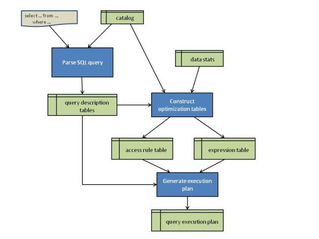
Figure 9 - RaimaDB SQL Query Optimization Process
Using the information in the catalog, the SELECT statement is parsed, validated, and represented in a set of easily processed query description tables. These tables include a tree representation of the WHERE clause expressions (called the expression tree) and information about the tables, columns, and keys in the database.
The system then analyzes those tables, and constructs both the access rule table and the expression table. For table that is referenced in the FROM clause, the analysis process uses information in the catalog and other data related statistics such as then number of rows in each table, blocking factors, and column distribution statistics. The access rule table contains a rule entry for each possible access method (for example, table scan or index lookup) for each table. The expression table has one entry for each conditional expression specified in the WHERE clause. These tables drive the actual optimization process.
Finally, the optimizer determines the plan with the lowest total cost. An execution plan basically consists of a series of steps (one step for each table listed in the FROM clause), of how the table in that particular plan step will be accessed. The possible access rules that can be applied at that step are sorted by their cost so that the first candidate rule is the cheapest. The optimizer's goal is to select one access rule for each step that minimizes the total cost of the complete execution plan. As the optimizer iterates through the steps, the cost of the candidate plan is updated. As soon as a candidate plan's cost exceeds the cost of the currently best complete plan, the candidate plan is abandoned at its current step and the next rule for that step is then tested. Conditional expressions that are incorporated into the plan are deleted from the expression tree so that they are not redundantly executed.